Anatomy of a Bullet Chart
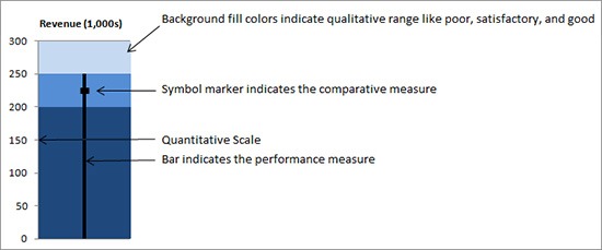
How to Make a Vertical Bullet Graph
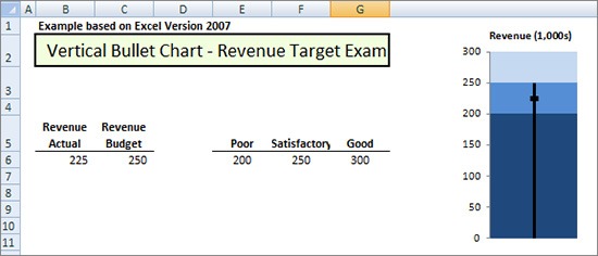
Making the Chart
Step 1: Create your chart. Select cells E5 through G6 and select the “Insert” tab and in the “Charts Section” click the down arrow under “Column” and select the first selection under 2-D bar for “Clustered Column” chart type.

Step 2: Delete the legend. Click the legend and press delete.

Step 3: Format rows and columns. Click the chart and select from “Chart Tools” tab and click “Switch Row/Column”.

Step 4: Overlap the data. Click the green bar and right click – a pop up box “Format Data Series” appears. Select “Series Options” (left side of the box) and in the right hand side under “Series Overlap” section move the arrow over to 100% overlapped and in the “Gap Width” section move the arrow over to “No Gap”. Click “Close”.
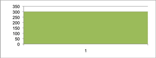
Step 5: Rearrange the bars. Click the green bar and under chart tools tab select “Select data”. Click the entry (Poor, Satisfactory, and Good) and use the up and down arrows located in the top right section on the “Legend Entries” box to move the entry up or down until you have “Good” on the top, “Satisfactory” and “Poor” at the bottom of the list. Click “OK”.

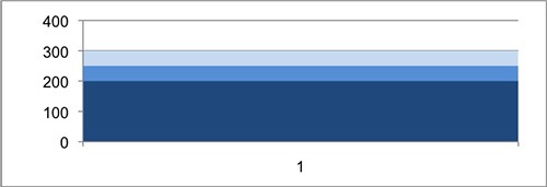
Step 6: Change the color of each of the bar sections to the same color in graduated sections. Right click on the blue section and select “Format Data Series”. Click on “Fill” in the left hand box inside the pop up window and then select “Solid Fill” in the right hand box and go down to the color icon and select the down arrow and select the darkest blue. Click “Close”. Repeat this step with the next two sections (red then green) selecting a lighter shade of blue each time to create a graduated color scheme.
Step 7A: Add Revenue Budget data (above in cells C5 and C6). Click the chart and then click the Chart Tools” tab at the top of the screen. Click “Select Data” and click the “Add” under “Legend Entries” to add National Average data. Under “Series Name” click the “spreadsheet icon” and then click on cell C5 above and click on the spreadsheet icon on the right hand side of the box and under “Series value” click on the “spreadsheet icon” and click cell C6 above and then click on the spreadsheet icon on the right hand corner of the box and then click on ‘OK”.
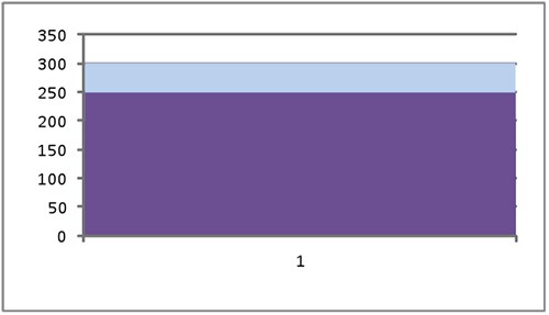
Step 7B: Add Revenue Actual data (above in cells B5 and B6). Click the chart and then click the Chart Tools” tab at the top of the screen. Click “Select Data” and click the “Add” under “Legend Entries” click “Add” and under “Series Name” click the “spreadsheet icon” and then click cell B5 (Actual) above and click on the spreadsheet icon on the right corner of the box and under “Series value” click the “spreadsheet icon” and then cell B6 above. Click on the spreadsheet icon on the right corner of the box. Click “OK”.
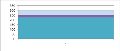
Step 8: Click the blue section of the graph and right click. A pop box will come up then select “Change Series Chart Type”. Select “XY Scatter” in the left hand section of the pop-up box. Select “Scatter with only markers”, which is the first selection under “XY Scatter” in the right hand section of the pop-up box. Click “OK”.
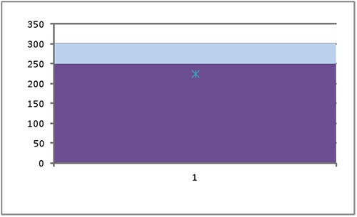
Step 9: Click on the purple section of the graph and right click. A pop box will come up, select “Change Series Chart Type”, select “XY Scatter” in the left hand section of the pop-up box, select “Scatter with only markers.” , which is the first selection under “XY Scatter” in the right hand section of the pop-up box. Click “OK”. You will end up with two X’s on the left hand axis of the graph.
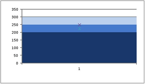
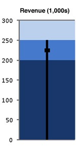
Step 10: Format into Bullet Graph. Click the first data point (225 value), select “Layout tab”, select “Error Bars” and select “Error Bars with Percentage”. You will end up with something that looks like a cross over the “X”.
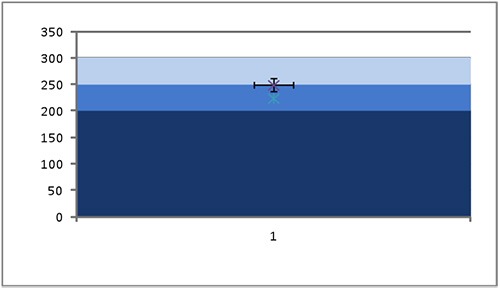
Step 11: Create Vertical Line. Click the horizontal part of the cross and press ‘delete’ which will leave you with vertical line over the “X”.
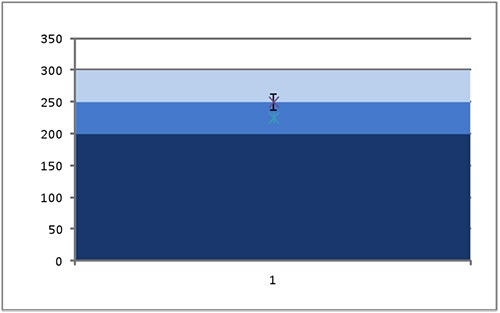
Step 12: Click the chart and then click the “Layout Tab” in the first section click the down arrow next to “Chart Area” and select “Series “Revenue Budget” Y Error Bars”. Click “Format Selection” and a pop up box appears. In the left hand side of the pop up box click “Vertical Error Bars” and in the right hand section, under “Display…Direction” click “Minus” and “Display…End Style”, click “No Cap”. Under ‘Error Amount’ click “Percentage” and change percentage to 100. Click “Line Style” in the left hand side under “Width” use the up arrow to change the “Width” to 3pt. to make a nice heavy line. Click “Close”.
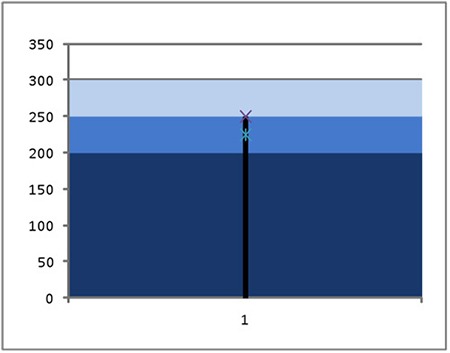
Step 13: Create Horizontal Line. Click the second data point, select Layout tab, select “Error Bars” and select “Error Bars with percentage”. You will end up with a cross over the “X”.
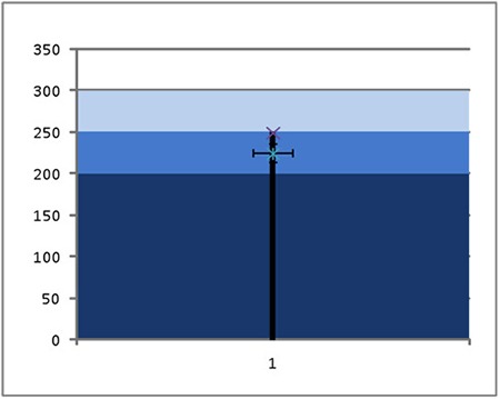
Step 14: Click the vertical part of the cross and press ‘delete’ which will leave you with horizontal line over the “X”.

Step 15: Click the chart and click on the Layout Tab under “Current Section” Click the down arrow next to “Chart Area” and select “Series “Revenue Actual X Error Bars” then click on ‘Format Selection” a pop up box comes up a In the left hand side of the pop up box click on “Horizontal Error Bars” and in the right hand section, under “Direction” click on “Both”. Under “End Style”, click on “No Cap”. Click on “Line Style” in the left hand side under “Width” use the up arrow to change the “Width” to 5 pt. to make a nice heavy line. Click “Close”.
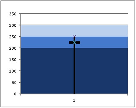
Step 16: Clean up Chart Junk. Select Markers from each of the lines by clicking the marker, right click and select “Format Data Series”. Select “Marker Options” and select None. Click “Close”. Click the Y axis and right click. Select “Format Axis”. Set the “Minimum” to 0 and “Maximum” to 300. Right click the x axis and press delete. Right click the chart and select “Format Chart Area” and select “Border Color” and click “No Line”. Click “Close”. To resize chart to desired size click the chart and drag the handles to the desired size.
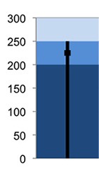
Step 17: Add a Title. Click on the chart and select “Layout Tab”. Click “Axis Titles”. Select “Primary Horizontal Axis Title” and click “Title Below Axis”.
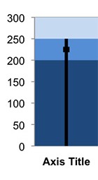
Step 18: Edit Title. Click on “Chart Title” and highlight the title and type Revenue (1,000s). Change the font size if necessary.
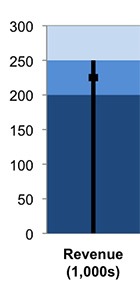
Step 19: Reposition Title to Top of Chart. Click on title and drag title to the top.


0 Comments